\(\renewcommand\AA{\unicode{x212B}}\)
Table of Contents
There are four QENS fitting interfaces:
These fitting interfaces share common features, with a few unique options in each.
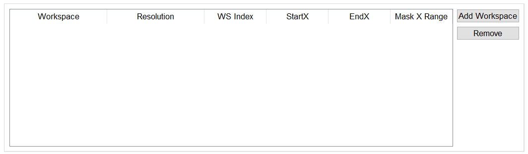
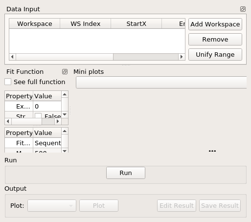
The input section for QENSFitting tabs consists of, a table along with two buttons ‘Add Workspace’ and ‘Remove’. Clicking ‘Add Workspace’ will allow you to add a new data-set to the fit (this will bring up a menu allowing you to select a file/workspace and the spectra to load). Once the data has been loaded, it will be displayed in the table. Highlighting data in the table and selecting ‘Remove’ will allow you to remove data from the fit. The Unify Range button changes the startX and endX values for all selected spectra in the table to be the same as the first spectra selected. Above the preview plots there is a drop-down menu with which can be used to select the active data-set, which will be shown in the plots.
There are options to fit your selected spectra either Sequentially or Simultaneously.
A sequential fit will fit each spectra one after another. By default this will use the end values of one fit as the starting values of the next. This behaviour can be toggled using the sequential/individual option.
A simultaneous fit will fit all the selected spectra against one cost function. The primary advantage of this method is that parameters which are expected to be constant across the data range can be tied across all the spectra. This leads to these parameters being fitted with better statistics and hence reduced errors.
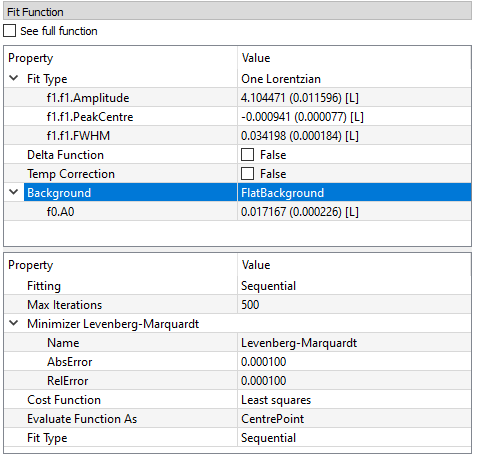
Under ‘Fit Function’, you can view the selected model and associated parameters as well as make modifications.
There are two modes which can be used to select functions. The default version allows easy selection of the most commonly used function models. The options in this mode differ for each of the four fitting tabs so more detailed information is given in the specific sections below. The other mode, which may be switched to bu ticking the See full function box, displays the generic function browser in which any function model can be specified.
Parameters may be tied by right-clicking on a parameter and selecting either ‘Tie > To Function’ to tie the parameter to a parameter of the same name in a different function, or by selecting ‘Tie > Custom Tie’ to tie to parameters of different names and for providing mathematical expressions. Parameters can be constrained by right-clicking and using the available options under ‘Constrain’.
Upon performing a fit, the parameter values will be updated here to display the result of the fit for the selected spectrum.
The bottom half of the Fit Function section contains a table of settings which control what sort of fit is done. These are:
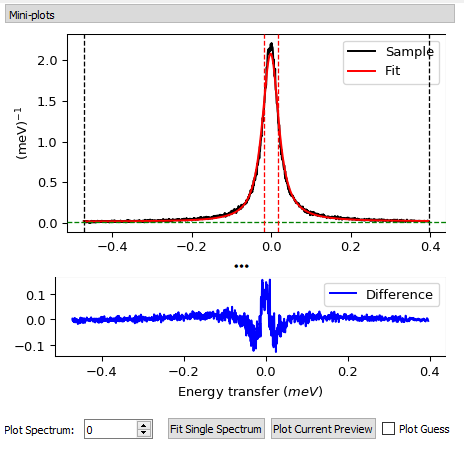
Two preview plots are included in each of the fitting interfaces. The top preview plot displays the sample, guess and fit curves. The bottom preview plot displays the difference curve.
The preview plots will display the curves for the selected spectrum (‘Plot Spectrum’) of the selected data-set (when in multiple input mode, a drop-down menu will be available above the plots to select the active data-set).
The ‘Plot Spectrum’ option can be used to select the active/displayed spectrum.
A button labelled ‘Fit Single Spectrum’ is found under the preview plots and can be used to perform a fit of the selected specturm.
‘Plot Current Preview’ can be used to plot the sample, fit, and difference curves of the selected spectrum in a separate plotting window.
The ‘Plot Guess’ check-box can be used to enable/disable the guess curve in the top preview plot.
The results of the fit may be plotted and saved under the ‘Output’ section of the fitting interfaces.
Next to the ‘Plot’ label, you can select a parameter to plot and then click ‘Plot’ to plot it with error bars across the fit spectra (if multiple data-sets have been used, a separate plot will be produced for each data-set). The ‘Plot Output’ options will be disabled after a fit if there is only one data point for the parameters.
During a sequential fit, the parameters calculated for one spectrum are used as the initial parameters for the next spectrum to be fitted. Although this normally yields better parameter values for the later spectra, it can also lead to poorly fitted parameters if the next spectrum is not ‘related’ to the previous spectrum. It may be useful to replace this poorly fitted spectrum with the results from a single fit using the ‘Edit Result’ option. Clicking the ‘Edit Result’ button will allow you to modify the data within your _Results workspace using the results produced from a fit to a single spectrum. See the algorithm IndirectReplaceFitResult.
Clicking the ‘Save Result’ button will save the result of the fit to your default save location.
Given either a saved NeXus file, or workspace generated using the Elwin tab, this tab fits \(intensity\) vs. \(Q\) with one of three functions for each run specified to give the Mean Square Displacement (MSD). It then plots the MSD as function of run number. This is done using the QENSFitSequential algorithm.
MSDFit searches for the log files named <runnumber>_sample.txt in your chosen raw file directory (the name ‘sample’ is for OSIRIS). These log files will exist if the correct temperature was loaded using SE-log-name in the Elwin tab. If they exist the temperature is read and the MSD is plotted versus temperature; if they do not exist the MSD is plotted versus run number (last 3 digits).
The fitted parameters for all runs are in _msd_Table and the <u2> in _msd. To run the Sequential fit a workspace named <inst><first-run>_to_<last-run>_eq is created, consisting of \(intensity\) v. \(Q\) for all runs. A contour or 3D plot of this may be of interest.
A sequential fit is run by clicking the Run button at the bottom of the tab, a single fit can be performed using the Fit Single Spectrum button underneath the preview plot. A simultaneous fit may be performed in a very similar fashion by changeing the Fit Type to Simultaneous and the clicking run.
The Peters model [1] reduces to a Gaussian at large (towards infinity) beta. The Yi Model [2] reduces to a Gaussian at sigma equal to zero.

The MSD Fit tab operates on _eq files. The files used in this workflow are produced on the Elwin
tab as seen in the Elwin Example Workflow.
osi104371-104375_graphite002_red_elwin_eq. Load this
file and it will be automatically plotted in the upper mini-plot.I(Q, t) Fit provides a simplified interface for controlling various fitting functions (see the Fit algorithm for more info). The functions are also available via the fit wizard.
The fit types available for use in IqtFit are Exponentials and Stretched Exponential.
The I(Q, t) Fit tab operates on _iqt files. The files used in this workflow are produced on the
I(Q, t) tab as seen in the I(Q, t) Example Workflow.
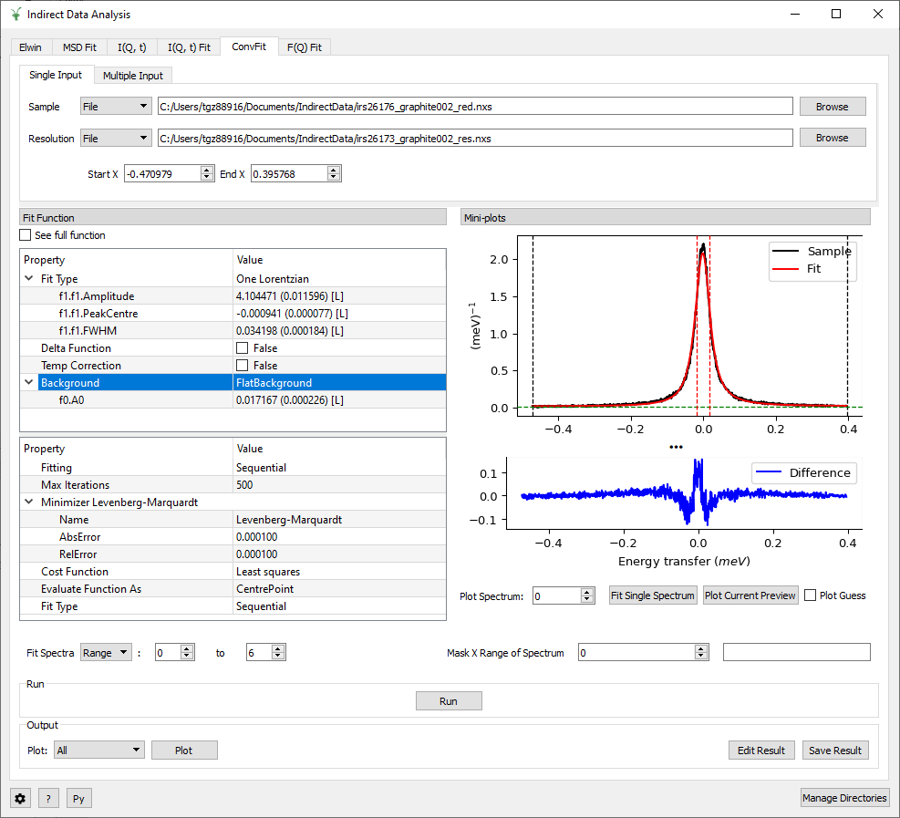
irs26176_graphite002_iqt.ConvFit provides a simplified interface for controlling various fitting functions (see the Fit algorithm for more info). The functions are also available via the fit wizard.
Additionally, in the bottom-right of the interface there are options for doing a sequential fit. This is where the program loops through each spectrum in the input workspace, using the fitted values from the previous spectrum as input values for fitting the next. This is done by means of the ConvolutionFitSequential algorithm.
A sequential fit is run by clicking the Run button at the bottom of the tab, a single fit can be done using the Fit Single Spectrum button underneath the preview plot.
The fit types available in ConvFit are One Lorentzian, Two Lorentzian, TeixeiraWater (SQE), InelasticDiffSphere, InelasticDiffRotDiscreteCircle, ElasticDiffSphere, ElasticDiffRotDiscreteCircle and StretchedExpFT.
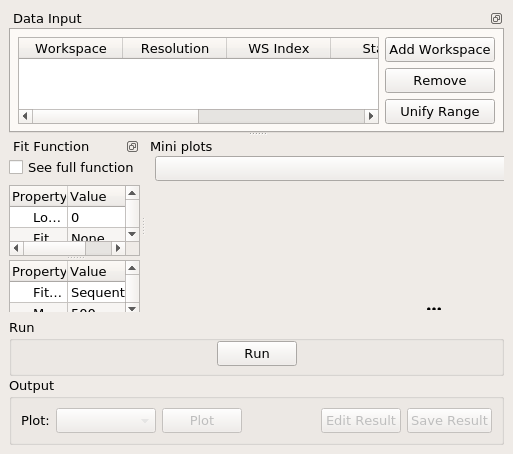
The Conv Fit tab allows _red and _sqw for its sample file, and allows _red, _sqw and
_res for the resolution file. The sample file used in this workflow can be produced using the run
number 26176 on the Indirect Data Reduction interface in the ISIS
Energy Transfer tab. The resolution file is created in the ISIS Calibration tab using the run number
26173. The instrument used to produce these files is IRIS, the analyser is graphite
and the reflection is 002.
iris26176_graphite002_red. Then click Browse
for the resolution and select the file iris26173_graphite002_res.The model used to perform fitting in ConvFit is described in the following tree, note that everything under the Model section is optional and determined by the Fit Type and Use Delta Function options in the interface.
The Temperature Correction is a UserFunction with the formula \(((x * 11.606) / T) / (1 - exp(-((x * 11.606) / T)))\) where \(T\) is the temperature in Kelvin.
One of the models used to interpret diffusion is that of jump diffusion in which it is assumed that an atom remains at a given site for a time \(\tau\); and then moves rapidly, that is, in a time negligible compared to \(\tau\).
This interface can be used for a jump diffusion fit as well as fitting across EISF. This is done by means of the QENSFitSequential algorithm.
The fit types available in F(Q)Fit are ChudleyElliot, HallRoss, FickDiffusion, TeixeiraWater, EISFDiffCylinder, EISFDiffSphere and EISFDiffSphereAlkyl.
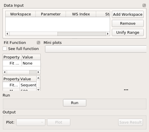
The F(Q) Fit tab operates on _result files which can be produced on the ConvFit tab. The
sample file used in this workflow is produced on the Conv Fit tab as seen in the
ConvFit Example Workflow.
irs26176_graphite002_conv_Delta1LFitF_s0_to_9_Result.There is the option to perform Bayesian data analysis on the I(Q, t) Fit ConvFit tabs on this interface by using the FABADA fitting minimizer, however in order to to use this you will need to use better starting parameters than the defaults provided by the interface.
You may also experience issues where the starting parameters may give a reliable fit on one spectra but not others, in this case the best option is to reduce the number of spectra that are fitted in one operation.
In both I(Q, t) Fit and ConvFit the following options are available when fitting using FABADA:
The FABADA minimizer can output a PDF group workspace when the PDF option is ticked. If this happens, then it is possible to plot this PDF data using the output options at the bottom of the tabs.
References
Categories: Interfaces | Indirect | Direct